Significance Tests for Covariates in LCA and LTA

I am performing LCA and wondered how to test the significance of my covariates. I understand that I need a test statistic and its corresponding degrees of freedom (df) to perform the test, but I don’t know how to get this information from my output. ––Signed, Feeling Insignificant

Dear F.I.,

A significance test can be helpful for judging whether there is sufficient evidence to state that a particular covariate is related to latent class membership. Significance tests provide p-values, which tell us how likely we would be to observe a relation between a covariate and latent class membership as strong as, or stronger than, the one in our sample, if in fact there is no relation between the two. A small p-value (say, p<.05) is generally taken as a relation being “statistically significant,” i.e., as evidence that a covariate is in fact related to latent class membership in the population. Follow these steps to test for statistical significance:

  1. Fit a model with the covariate of interest; save the loglikelihood as ‘alt_loglike.’
  2. Fit a model with the covariate removed; save the loglikelihood as ‘null_loglike.’
  3. Compute the likelihood ratio test statistic: ‘delta_2ll = 2(alt_loglike – null_loglike).’
  4. Determine the df for the likelihood ratio test by determining how many additional parameters are estimated in Step 1 compared to Step 2. This is easily done by counting up the number of additional regression coefficients estimated in Step 1 compared to Step 2. Because the intercept coefficients are estimated in both the null and the alternative models, they do not need to be counted; that is, only the “slope parameters” need to be counted.For example, for LCA with multinomial logistic regression, df = (number of latent classes – 1) * (number of groups). This is because the model with the covariate (in Step 1) estimates an additional slope parameter, compared to the model without the covariate (in Step 2), for the effect of the covariate on each latent class compared to a reference latent class, within each group. For LCA with binary logistic regression, df = (number of groups). This is because the model with the covariate estimates one additional slope parameter, compared to the model without the covariate, for the effect of the covariate on a target latent class compared to all other latent classes combined for the reference, within each group. Remember that in LTA many more slope parameters are estimated when you predict transitions; be sure to count them all.
  5. Evaluate the cumulative distribution function of a chi-square distribution for the value ‘delta_2ll’ with the corresponding df. This is the p-value for that covariate. You can use an online calculator for this computation.

For example, there is a high-quality online calculator here. Using this calculator, you would put in ‘delta_2ll’ for X2 and ‘df’ for d. The calculator then reports the p-value for you.

Good luck in your research!

Bethany Bray

LCA vs Factor Analysis: About Indicators

My understanding is that when an indicator has no relation to the latent construct of interest, this is represented differently in LCA than in factor analysis. Can you explain how and why this works? ––Signed, Latently Lost

Dear Lost,

In factor analysis, factor loadings are regression coefficients, so a factor loading of zero represents “no relation” between the manifest indicator and the latent factor, whereas factor loadings closer to -1 and 1 represent stronger relations. In comparison, in latent class analysis, item-response probabilities play the same conceptual role as factor loadings, but they are conditional probabilities, not regression coefficients. Item-response probabilities closer to 0 and 1 represent stronger relations between the manifest indicator and latent class variable. The closer item-response probabilities are to 1/(marginal probability) for all classes, the weaker the relation between the manifest variable and the latent class variable. “High homogeneity” refers to the degree to which item-response probabilities are close to 0 and 1 in latent class analysis; this concept is similar to the concept of “saturation” in factor analysis.

Ideally, the pattern of item-response probabilities also clearly identifies latent classes with distinguishable interpretations; this concept of “latent class separation” is similar to the concept of “simple structure” in factor analysis. When model selection is difficult due to conflicting information from fit criteria, the concepts of homogeneity and latent class separation can be a helpful way to approach model selection based on relevant theory from your specific field.

Happy analyzing!

Bethany Bray

Factorial Experiments

I am interested in Dr. Collins’ work on optimizing behavioral interventions, and I was surprised that she advocates the use of factorial experimental designs for some experiments. I was taught that factorial experiments could never be sufficiently powered. Can factorial designs really be implemented in practice? — Signed, Fretting Loss of Power

Dear FLOP,

This is a common question. Experimental subjects are often expensive or scarce. In these cases, a factorial experiment can save money and resources and still provide sufficient statistical power.

Dr. Welton is revamping a high-risk teen drinking intervention to be delivered in mental health settings, and she is deciding which of the following components to add: (A) peer-based sessions; (B) parent-based sessions; (C) drug resistance skills; and/or (D) drug use education. Dr. Welton wants to decide which combination of the new components will achieve the best participant adherence. Dr. Welton considers two different design approaches:

  1. Conduct four separate experiments, one corresponding to each of the intervention components. Each experiment would involve two conditions: (i) a condition in which the intervention component is included, and (ii) a control condition in which the intervention component is not included. For each of the four experiments, the data analysis would produce an estimate of the mean difference between the two conditions.
  2. Conduct a factorial experiment. This approach would treat each of the four components as a factor (i.e., independent variable) that can take on the levels “not included” or “included.” Crossing these factors would result in 16 experimental conditions (every combination of the levels of the four factors) and provide estimates of the main effect of each component and all interactions between components.

Next, Dr. Welton considers the cost of each approach. She anticipates a per-subject cost of $100. In addition, the overhead associated with each experimental condition (except for the control condition) will be $500, which is the cost of developing materials and training staff for each new version of the intervention. She specifies that each component has to produce an effect of at least .35 of a standard deviation in order to be considered for inclusion in the new intervention. Therefore, Dr. Welton wants to be sure she has the power to detect effects of at least this size.

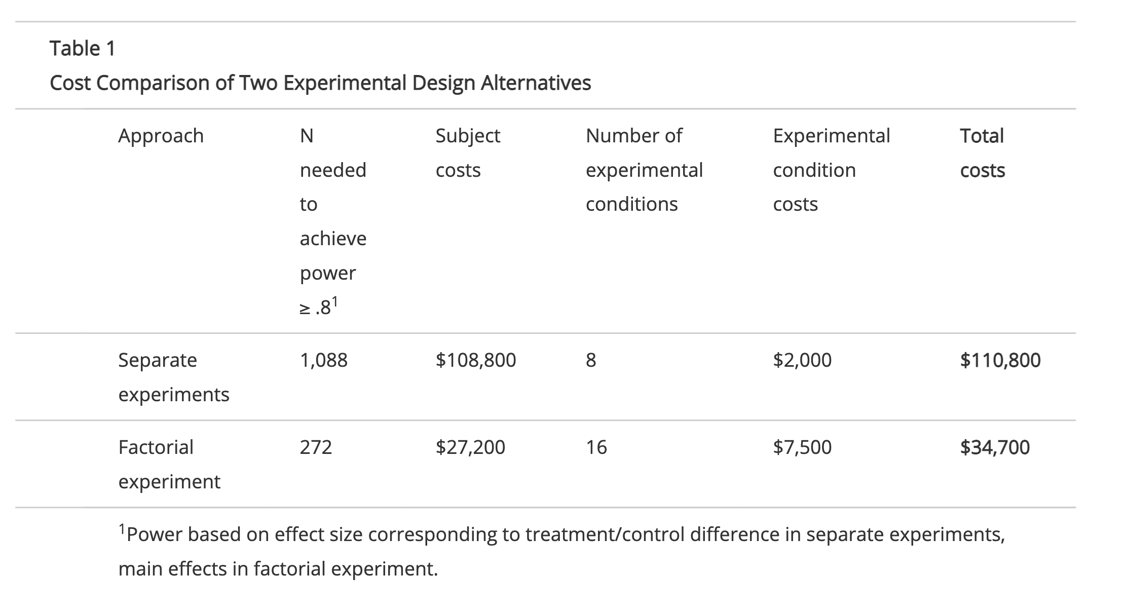
Table 1 compares the cost of each approach. To achieve the desired statistical power in this example, the separate experiments approach requires four times as many subjects as the factorial experiment. Dr. Welton would save $76,100 by conducting a factorial experiment instead of four separate experiments! Collins, Dziak, and Li (2009) discuss how to determine which of several design alternatives is most cost-effective in a given situation. A free SAS macro for comparing the relative costs of a variety of experimental designs can be found here.

Analyzing EMA Data

I designed a study to assess 50 college students’ motivations to use alcohol and its correlates during their first semester. The most innovative part of this study was that I collected data with smart phones that beeped at several random times on every Thursday, Friday, and Saturday throughout the semester. Now that I’ve collected the data, I’m overwhelmed by how rich the data are and don’t know where to start! My first thought is to collapse the data to weekly summary scores and model those using growth curve analysis. Is there anything more I can do with the data? — Signed, Swimming in Data

Dear Swimming:

You did indeed collect an amazing dataset! With technological advances, the collection of intensive longitudinal data, such as ecological momentary assessments (EMA), is becoming popular among researchers hoping to better understand dynamic processes related to mood, cigarette or alcohol use, physical activity, and many other states or behaviors. Some of the most compelling research questions in these studies often have to do with effects of time-varying predictors.

One familiar way to approach the analysis of EMA data is to reduce the data, summarizing within-day or within-week assessments to a single measure, so that growth curve models may be fit to estimate an average trend and predictors of the intercept and slope. However, this approach disregards the richness of the data that were so carefully collected. Further, EMA studies are typically designed in order to capture something more dynamic than what could be captured as a linear function of time.

A more common approach to the analysis of EMA data is multilevel models, where within- and between-individual variability can be separated. This approach is helpful for understanding, for example, the degree of stability of processes. However, these methods typically impose important constraints, such as the assumption that the effects of covariates on an outcome are stable over time.

New methods for the analysis of intensive longitudinal data have been proposed in the statistical literature, and hold immense promise for addressing important questions about dynamic processes such as the factors driving alcohol use during the freshman year of college. For example, the time-varying effect model (TVEM) is a flexible approach that allows the effects of covariates to vary with time. A detailed introduction to time-varying effect models for audiences in psychological science will appear in Tan, Shiyko, Li, Li, & Dierker (in press).

A demonstration of this approach will appear in an article by Methodology Center researchers and colleagues (Shiyko et al., in press). The authors analyzed data collected as part of a smoking-cessation trial and found that individuals with a successful quit attempt had a rapid decrease in craving within the first few days of quitting, whereas those who eventually relapsed did not experience this decrease. Eventual relapsers had low levels of confidence in their abilities to abstain on cravings early in their quit attempt, but among successful quitters the association with confidence in ability to abstain was significantly weaker.

Any researcher with access to EMA data can fit a TVEM using the %TVEM SAS macro, which is freely available at /downloads/tvem. Give it a try so that you can explore the timevarying effects of individual factors, such as residing in a dorm, and contextual factors, such as excitement about an upcoming sporting event, on motivations to use alcohol.

References

Shiyko, M. P., Lanza, S. T., Tan, X., Li, R., & Shiffman, S. (2012). Using the time-varying effect model (TVEM) to examine dynamic associations between negative affect and self confidence on smoking urges: Differences between successful quitters and relapsers. Prevention Science. PMCID: PMC3171604

Tan, X., Shiyko, M. P., Li, R., Li, Y., & Dierker, L. (2012). A time-varying effect model for intensive longitudinal data. Psychological Methods, 17(1), 61-77. PMCID: PMC3288551

Are Adaptive Interventions Bayesian?

I love the idea of adaptive behavioral interventions. But, I keep hearing about adaptive designs and how they are Bayesian. How can an adaptive behavioral intervention be Bayesian? —Signed, Adaptively Confused, Determined to Continue

Dear AC, DC:

Actually, adaptive behavioral interventions are not Bayesian, but your confusion is understandable, because the same words have been used to refer to different concepts.

Let’s start with the word “adaptive.” This word, which is used in many fields, refers broadly to anything that changes in a principled, systematic way in response to specific circumstances in order to produce a desired outcome. An adaptive intervention is a set of tailoring variables and decision rules whereby an intervention is changed in response to characteristics of the individual program participant or the environment in order to produce a better outcome for each participant (Collins et al., 2004). For example, in an adaptive intervention for treating alcoholism, an individual participant’s alcohol intake may be monitored and reviewed periodically. Here alcohol intake is the tailoring variable. The decision rule might be as follows: if the individual has no more than two drinks per week for six weeks, frequency of clinic visits will be reduced. On the other hand, if the individual has more than two drinks per week, additional clinic visits will be required, plus a pharmaceutical will be added to the treatment regime.

Now let’s discuss the word “design.” In intervention science, the term intervention design refers to the specifics of a behavioral intervention: the factors included in the prevention or treatment approach, such as whether the intervention is delivered in a group or individual setting, or the intensity level of the intervention. In contrast, the term research design refers to how an empirical study is set up. For example, in an experimental research design there is random assignment to conditions; in a longitudinal research design, measures are taken over several different time points.

Confusion may arise when the words “adaptive” and “design” are paired without specifying which sense of the word “design” is meant. In intervention science, an adaptive intervention design is the approach used in a particular adaptive intervention. In methodology, an adaptive research design (Berry et al., 2011) is a Bayesian approach to randomized clinical trials (RCTs), in which the research design may be altered during the course of a clinical trial based on information gathered during the trial. For example, an adaptive clinical trial may be halted before the entire planned sample size is collected if the results are judged to be so clear that additional information would be unlikely to affect decision making. Adaptive intervention designs are not experimental designs, and therefore cannot be Bayesian.

You might think that building or evaluating an adaptive behavioral intervention would require the use of an adaptive experimental design, but this is generally not the case. Investigators who want to build an adaptive intervention—that is, conduct an experiment to decide on the best tailoring variables and/or decision rules—probably want to consider a Sequential Multiple Assignment Randomized Trial (SMART Trial; Murphy et al., 2007). Note that the SMART Trial has been developed especially for building adaptive behavioral interventions, but it is not an adaptive experimental design.

Investigators who have already selected the tailoring variables and decision rules and want to evaluate the adaptive intervention probably want to conduct an RCT. The RCT could potentially involve an adaptive experimental design, but it could also be a standard RCT.

I hope this helps to clear things up! Reading the references listed below may help. And, AC, DC: The next time you hear the term “design,” if you are not sure whether the speaker is talking about intervention design or experimental design, be sure to ask forc larification.

References

Berry, S. M., Carlin, B. P., Lee, J. J., & Muller, P. (2011). Bayesian adaptive methods for clinical trials. Boca Raton, FL: CRC Press.

Collins, L. M., Murphy, S. A., & Bierman, K. (2004). A conceptual framework for adaptive preventive interventions. Prevention Science, 3, 185-196

Murphy, S. A., Lynch, K. G., McKay, J. R., Oslin, D., & Ten Have, T. (2007). Developing adaptive treatment strategies in substance abuse research. Drug and Alcohol Dependence, 88(2), S24-S30.

Modeling Multiple Risk Factors

I want to investigate multiple risk factors for health risk behaviors in a national study, but do not know how to handle the high levels of covariation among the different risk factors. Do you recommend that I regress the outcome on the entire set of risk factors using multiple regression analysis? Or should I create a cumulative risk index by summing risk exposure, and regress the outcome on that index? — Signed, Waiting to Regress

Dear WTR,

Recognizing that individuals develop within multiple contexts, and therefore simultaneously can be exposed to numerous—often highly correlated—risk factors, is critical in studies of human behavior and development. Historically, multiple risks for a poor outcome have typically been modeled using two approaches: multiple regression analysis and/or a cumulative risk index.

Multiple regression allows us to examine the relative importance of each risk factor in predicting the outcome, but there can be drawbacks: without the inclusion of many higher-order interactions, it is impossible to examine how exposure to certain combinations of risk factors impacts the outcome. Also, high levels of multicollinearity (for example, among risk factors such as maternal education, neighborhood disorganization, and residential crowding) can severely distort inference based on multiple regression.

Alternatively, a cumulative risk index can be created by summing for each individual the number of risk factors to which they are exposed. Instead of regressing the outcome on all individual risk factors, the outcome is simply regressed on the index score. Early work in this area represented an important step forward in thinking about multiple risks. A downside to this approach is that each risk factor is equally weighted; this means that exposure to each additional risk factor (regardless of which one) corresponds to an equal level of increased risk. Furthermore, such an index does not provide any insight into how particular risk factors co-occur or interact with each other.

A person-centered approach to modeling multiple risks was recently demonstrated by Lanza and colleagues (Lanza, Rhoades, Nix, Greenberg, and CPPRG, 2010). This study used latent class analysis to identify four unique risk profiles based on exposure to thirteen risk factors across child, family, school, and neighborhood domains. Each risk profile characterized a unique group of children: (1) Two-Parent Low Risk, (2) Single Parent with a History of Problems, (3) One-Parent Multilevel Risk, and (4) Two-Parent Multilevel Risk. Compared to a cumulative risk index, an examination of the link between risk profile membership during kindergarten and externalizing problems, school failure, and low academic achievement in fifth grade provided a more nuanced understanding of the early precursors to negative outcomes. The application of latent class analysis to multiple risks holds promise for informing the refinement of preventive interventions for groups of children who share particular combinations of risk factors.

Reference

Lanza, S. T., Rhoades, B. L., Nix, R. L., Greenberg, M. T., & The Conduct Problems Prevention Research Group (2010). Modeling the interplay of multilevel risk factors for future academic and behavior problems: A person-centered approach. Development and Psychopathology, 22, 313-335.

Handling Time-Varying Treatments

I’ve heard about new methodologies being developed that allow scientists to address novel scientific questions concerning the effects of time-varying treatments or predictors using observational longitudinal data. What are some examples of these scientific questions, and where can I read up on these newer methodologies? —Signed, Time for a Change

Dear TFAC,

Scientists often have longitudinal data that includes time varying covariates, time-varying treatments (or time varying predictors of interest), and longitudinal outcomes. In these settings, scientists may examine a varied number of scientific questions having to do with the impact of additional treatment, the effect of treatment sequences,timing, or treatment duration. One example involves understanding the effect of a putative moderator when both the moderator and primary treatment variable are time-varying. For instance, the following set of questions examine whether baseline and intermediate severity is a time-varying moderator (Almirall, Ten Have et al. 2009; Almirall, McCaffrey et al. under review) of the effect of community-based substance abuse treatment:

(a) “What is the effect of receiving an initial 3 months of community-based substance abuse treatment on substance use frequency among adolescents with less versus more severity at intake (baseline)?” and

(b) “What is the effect of receiving an additional 3 months of treatment some time later, as a function of improvements in severity since intake?”

In the time-varying setting, standard regression approaches that naively adjust for time-varying covariates may not be appropriate, and, in fact, may cause additional bias (Almirall, Ten Have et al. 2009; Almirall, McCaffrey et al. under review; Barber, Murphy et al. 2004; Bray, Almirall et al. 2006; Robins, Hernan et al. 2000). In the example given above, for instance, adjusting for time-varying severity is problematic because intermediate severity may have been affected by treatment during the first 3 months (this may happen, for example, if intermediate severity is a mediator of the effect of earlier treatment on future substance use frequency). Two problems with the traditional regression approach—both of which stem from adjusting for time-varying covariates possibly affected by earlier treatment—are described conceptually in Almirall, McCaffrey, et al (under review) in the context of a substance abuse example. Their article also offers a new 2-stage regression-with-residuals approach to examining the effect of time-varying treatments or predictors; the new approach involves a relatively simple adaptation of the traditional regression approach.

References

Almirall, D., McCaffrey, D. F., Ramchand, R., & Murphy,S. A. (under review). Subgroups analysis when treatment and moderators are time-varying.

Almirall, D.,Ten Have,T. R., & Murphy, S. A. (in press). Structural nested mean models for assessing time-varying effect moderation. Biometrics.

Barber, J. S., Murphy, S. A., & Verbitsky, N. (2004). Adjusting for time-varying confounding in survival analysis. Sociological Methodology, 34, 163-192.

Bray, B. C., Almirall, D., Zimmerman, R. S., Lynam, D., & Murphy, S. A. (2006). Assessing the total effect of time-varying predictors in prevention research. Prevention Science 7, 1-17.

Robins, J. M., Hernan, M. A., & Brumback, B. (2000). Marginal structural models and causal inference in epidemiology. Epidemiology 11, 550-560.

Experimental Designs That Use Fewer Subjects

I am trying to develop a drug abuse treatment intervention. There are six distinct components I am considering including in the intervention. I need to make the intervention as short as I can, so I don’t want to include any components that aren’t having much of an effect. I decided to conduct six experiments, each of which would examine the effect of a single intervention component. I need to be able to detect an effect size that is at least d =.3; any smaller than that and the component would not be pulling its own weight, so to speak. I have determined that I need a sample size of about N=200 for each experiment to maintain power at about .8. But then I did the math and figured out that with six experiments, I would need 6 X 200 = 1200 subjects! Yikes! Is there any way I can learn what I need to know, but using fewer subjects? —Signed, Experimental Design Gives Yips

Dear EDGY, Have you considered examining all six components in a single factorial experiment? If you did this, you would need only 200 subjects total to maintain power at .8 for testing the main effect of each component. This experiment would have 26=64 experimental conditions, with only a few subjects per condition. (In practice, you might want to use either 192 or 256 subjects so you could have equal numbers of subjects in each condition.) Unlike the approach of separate individual experiments, this factorial experiment would enable estimation of interactions.

Of course, an important question is whether it is feasible for you to implement 64 experimental conditions.You do not mention the context in which you are conducting this research. For example, if this is an internet-delivered intervention, 64 conditions may be feasible.

If it is not feasible for you to conduct an experiment with 64 conditions, but you would nevertheless like to take advantage of the economy associated with factorial experiments, you may want to consider conducting a fractional factorial experiment. Fractional factorial designs are used commonly in engineering. In general, these designs are most useful when there is no a prior reason to believe that the higher-order interactions are sizeable. There are a lot of different fractional factorial designs to choose from, each representing a different set of trade-offs between efficiency and assumptions. For example, with six independent variables there is a fractional factorial design available to you that would involve only 16 experimental conditions. This design would enable you to estimate all six main effects, and requires the assumption that all interactions three-way and higher are negligible. This design has the same sample size requirements as the complete factorial experiment, that is, N=200 to maintain power at .8. Other fractional factorial designs are available to you that require less stringent assumptions.

For a comparison of the economy of factorial experiments vs. individual experiments, and a brief tutorial on fractional factorial designs, see Collins, Dziak, and Li (2009).

Reference

Collins, L. M., Dziak, J. J., & Li, R. (2009). Design of experiments with multiple independent variables: a resource management perspective on complete and reduced factorial designs. Psychological methods, 14(3), 202.

Fit Statistics and SEM

I am interested in examining the role of three variables (family drug use, family conflict and family bonding) as mediators of the effect of neighborhood disorganization on adolescent drug use. I fit a structural equation model, but wonder which of the many fit statistics I should report?— Signed, Befuddled by Fit

Dear Befuddled,

Generally, in structural equation modeling you should report several fit indices rather than only one. More specifically, simulation studies have shown that the Relative Normed Index and the Comparative Fit Index are both essentially unbiased (that is, they correctly estimate what the fit would be if the model were fit to the whole population).

Coffman (2008) found that the RMSEA was biased in most conditions; specifically, she found that this fit statistic underestimated the population value, which means that investigators would be more likely to conclude that their model fits when in some cases it does not. However, she found that the RMSEA confidence interval maintained 95% coverage, which is a very desirable characteristic. In other words, she found in a simulation study that roughly 95/100 times the RMSEA confidence interval contained the true population value of the RMSEA. This means that the Type I error rate based on the confidence intervals matched the specified alpha of .05. In addition, both the test of exact fit (i.e. RMSEA = 0) and the test of close fit (e.g. RMSEA < .05) based on these confidence intervals worked well in terms of Type I error rates and power.

Based on these findings, I recommend reporting either the Relative Normed Index or the Comparative Fit Index (since these two indices are quite similar), along with the RMSEA confidence interval, noting its width and the upper bound of the interval.

Reference

Coffman, D.L. (2008). Model misspecification in covariance structure models: Some implications for power and Type I error. Methodology, 4(4), 159-167.

Modeling Behavior Change Over Time

I am interested in modeling change over time in risky sexual behavior during adolescence, but I cannot decide how to code my outcome variable. I could create a dummy variable at each time point that indicates whether or not the individual has had intercourse, a count variable for the number of partners, or a continuous measure of the proportion of times they used a condom, but none of these approaches seems to capture the complex nature of the behavior. — Uni Dimensional

Dear Uni,

You are right that all of these dimensions (having intercourse, number of partners, proportion of times used a condom) may be important to take into account in a model of sexual risk behavior. It’s difficult to imagine a single composite score that could reflect these different aspects of behavior. One approach you might consider is modeling the outcome as a latent class variable. Latent class analysis (LCA) is a measurement model that identifies underlying subgroups in a sample based on a set of categorical indicators. In your study, each indicator can correspond to a different dimension or aspect of behavior. This approach would yield a set of subgroups of individuals, each characterized by a particular behavioral pattern. Although each individual’s true class membership is unknown, the model provides estimates of an individual’s probability of membership in each class.

Latent class analysis can be extended to longitudinal data. This approach, called latent transition analysis (LTA), is used to estimate transitions over time in latent class membership. In other words, development in discrete latent variables over two or more times can be examined. Once a latent transition model is selected, covariates can be incorporated in the model as predictors of initial status or as predictors of change over time in the behavior. This would allow you to address questions such as “Does parental permissiveness in middle school predict sexual behavior in middle school, or transitions to more risky behavior in high school?” In addition, the model can be extended to include multiple groups in order to determine whether characteristics such as ethnicity moderate the relation between parental permissiveness and transitions to more risky behavior.

Lanza & Collins (2008) demonstrated the use of latent transition analysis to model change over time in dating and sexual risk behavior across three time points during emerging adulthood. Data were from three waves of the National Longitudinal Survey of Youth 1997. Four categorical indicators of the latent variable were assessed each year: the number of dating partners in the past year (0, 1, 2 or more), past-year sex (yes, no), the number of sexual partners in the past year (0, 1, 2 or more), and unsafe sex, that is, sex without a condom, in the past year (yes, no). The following five latent classes were identified at each time: Non-daters(18.6% at Time 1), Daters (28.9%), Monogamous (11.7%), Multi-partner safe (23.1%), and Multi-partner exposed (17.7%). Transition probabilities showed that members of the higher-risk Multi-partner exposed latent class were most stable in their behavior across time. Interestingly, individuals who were most likely to transition into this higher-risk latent class were members of the Monogamous latent class, suggesting that the Monogamous group might be an important target for prevention efforts. Alcohol, cigarette, and marijuana use all were significantly related to sexual risk behavior at Time 1, although alcohol and marijuana use were stronger predictors of membership in the higher-risk Multi-partner exposed latent class than cigarette use. Past-year drunkenness predicted transitions from the Non-daters and Daters latent classes to the Multi-partner exposed latent class.

PROC LCA & PROC LTA, SAS procedures for latent class and latent transition analysis, are available free of charge from The Methodology Center website.

Reference

Lanza, S. T., & Collins, L. M. (2008). A new SAS procedure for latent transition analysis: Transitions in dating and sexual risk behavior. Developmental Psychology, 44(2) 446-456.

Propensity Scores

I have been hearing a lot lately about propensity scores. What are they, and how can I use them? — Signed, Lost Cause

Dear Lost,

Propensity scores are useful when trying to draw causal conclusions from observational studies where the “treatment” (i.e. the “independent variable” or alleged cause) was not randomly assigned. For simplicity, let’s suppose the treatment variable has two levels: treated (T=1) and untreated (T=0). The propensity score for a subject is the probability that the subject was treated, P(T=1). In a randomized study, the propensity score is known; for example, if the treatment was assigned to each subject by the toss of a coin, then the propensity score for each subject is 0.5. In a typical observational study, the propensity score is not known, because the treatments were not assigned by the researcher. In that case, the propensity scores are often estimated by the fitted values (p-hats) from a logistic regression of T on the subjects’ baseline (pre-treatment) characteristics.

In an observational study, the treated and untreated groups are not directly comparable, because they may systematically differ at baseline. The propensity score plays an important role in balancing the study groups to make them comparable. Rosenbaum and Rubin (1983) showed that treated and untreated subjects with the same propensity scores have identical distributions for all baseline variables. This “balancing property” means that, if we control for the propensity score when we compare the groups, we have effectively turned the observational study into a randomized block experiment, where “blocks” are groups of subjects with the same propensities.

You may be wondering: why do we need to control for the propensity score, rather than controlling for the baseline variables directly? When we regress the outcome on T and other baseline characteristics, the coefficient for T is an average causal effect only under two very restrictive conditions. It assumes that the relations between the response and the baseline variables are linear, and that all of the slopes are the same whether T=0 or T=1. More elaborate analysis of covariance (ANCOVA) models can give better results (Schafer & Kang, under review), but they make other assumptions. Propensity scores provide alternative ways to estimate the average causal effect of T without strong assumptions about how the response is related to the baseline variables.

So, how do we use the propensity scores to estimate the average causal effect of T? Because the propensity score has the balancing property, we can divide the sample into subgroups (e.g., quintiles) based on the propensity scores. Then we can estimate the effect of T within each subgroup by an ordinary t-test, and pool the results across subgroups (Rosenbaum & Rubin, 1984). Alternatives to subclassification include matching and weighting. In matching, we find a subset of untreated individuals whose propensity scores are similar to those of the treated persons, or vice-versa (Rosenbaum, 2002). In weighting, we compare weighted averages of the response for treated and untreated persons, weighting the treated ones by 1/P(T=1) and the untreated ones by 1/P(T=0) (Lunceford & Davidian, 2004). However, very large weights can make estimates unstable.

References

Lunceford, J. K., & Davidian, M. (2004). Stratification and weighting via the propensity score in estimation of causal treatment effects: A comparative study. Statistics in Medicine, 23, 2937-2960.

Rosenbaum, P. R., & Rubin, D. B. (1983). The central role of the propensity score in observational studies for causal effects. Biometrika, 70(1), 41-55.

Rosenbaum, P. R., & Rubin, D. B. (1984). Reducing bias in observational studies using subclassification on the propensity score. Journal of the American Statistical Association, 79, 516-524.

Rosenbaum, P. R. (2002). Observational Studies, 2nd Edition. New York: Springer Verlag.

Schafer, J. L., & Kang, J. D. Y. (under review). Average causal effects: A practical guide and simulated case study.

AIC vs. BIC

I often use fit criteria like AIC and BIC to choose between models. I know that they try to balance good fit with parsimony, but beyond that I’m not sure what exactly they mean. What are they really doing? Which is better? What does it mean if they disagree? — Signed, Adrift on the IC’s

Dear Adrift,

As you know, AIC and BIC are both penalized-likelihood criteria. They are sometimes used for choosing best predictor subsets in regression and often used for comparing nonnested models, which ordinary statistical tests cannot do. The AIC or BIC for a model is usually written in the form [-2logL + kp], where L is the likelihood function, p is the number of parameters in the model, and k is 2 for AIC and log(n) for BIC.

AIC is an estimate of a constant plus the relative distance between the unknown true likelihood function of the data and the fitted likelihood function of the model, so that a lower AIC means a model is considered to be closer to the truth. BIC is an estimate of a function of the posterior probability of a model being true, under a certain Bayesian setup, so that a lower BIC means that a model is considered to be more likely to be the true model. Both criteria are based on various assumptions and asymptotic approximations. Each, despite its heuristic usefulness, has therefore been criticized as having questionable validity for real world data. But despite various subtle theoretical differences, their only difference in practice is the size of the penalty; BIC penalizes model complexity more heavily. The only way they should disagree is when AIC chooses a larger model than BIC.

AIC and BIC are both approximately correct according to a different goal and a different set of asymptotic assumptions. Both sets of assumptions have been criticized as unrealistic. Understanding the difference in their practical behavior is easiest if we consider the simple case of comparing two nested models. In such a case, several authors have pointed out that IC’s become equivalent to likelihood ratio tests with different alpha levels. Checking a chi-squared table, we see that AIC becomes like a significance test at alpha=.16, and BIC becomes like a significance test with alpha depending on sample size, e.g., .13 for n = 10, .032 for n = 100, .0086 for n = 1000, .0024 for n = 10000. Remember that power for any given alpha is increasing in n. Thus, AIC always has a chance of choosing too big a model, regardless of n. BIC has very little chance of choosing too big a model if n is sufficient, but it has a larger chance than AIC, for any given n, of choosing too small a model.

So what’s the bottom line? In general, it might be best to use AIC and BIC together in model selection. For example, in selecting the number of latent classes in a model, if BIC points to a three-class model and AIC points to a five-class model, it makes sense to select from models with 3, 4 and 5 latent classes. AIC is better in situations when a false negative finding would be considered more misleading than a false positive, and BIC is better in situations where a false positive is as misleading as, or more misleading than, a false negative.

Evaluating Latent Growth Curve Models

I am using a latent growth curve approach to model change in problem behavior across four time points. Although my exploratory analyses suggested that a linear growth function would describe individual trajectories well for nearly all of the adolescents in my sample, the overall model fit (in terms of RMSEA and CFI) is poor. Is my model really that bad? — Signed, Fit to be Tied

Dear Fit,

The overall fit statistics for latent growth curve models assess the fit of the covariance structure as they do for any structural equation model. Although they are informative, they do not provide information about the fit of the functional form, the fit of individual trajectories, or the fit of the mean structure. Generally, one is interested in either the difference between the group mean trajectory and an individual’s observed trajectory or the difference between an individual’s observed trajectory and the same individual’s model implied (or predicted) trajectory. The former provides a method for detecting outliers whereas the latter provides a method for assessing the fit of individual trajectories.

The former is quantified in the individual loglikelihoods which, when summed over the entire sample, add up to the overall log-likelihood. Further details about individual log-likelihoods in the context latent growth curve models may be found in Coffman and Millsap (2006). For cases with large individual log-likelihood values, the lack of fit may be due to either incorrect functional form or the case may lie far from the group mean trajectory. Examining a plot of the individual’s observed trajectory provides an indication as to the reason for the lack of fit.

The difference between an individual’s observed trajectory and the same individual’s predicted trajectory is more difficult to quantify. This is because in the framework of factor analysis, the individual’s predicted trajectory is based on factor scores. These are not estimated as part of fitting the model and within the factor analysis tradition are considered indeterminate. Thus, there are several methods for obtaining these predicted trajectories, each leading to different predictions. Once a method for computing the predicted trajectories has been chosen, then one could summarize the difference between the predicted trajectory and the observed trajectory as a root mean square residual between the predicted and observed values for an individual.

It is important to note that examining the fit using individual log-likelihoods may be done only when there are no data missing. This is because individuals with more missing data will contribute less to the overall log-likelihood (their individual log-likelihood will be smaller) than those with less missing data. This may lead to the conclusion that a particular individual does not fit as well when in fact the individual’s log-likelihood is larger due to the absence of missing data.

Reference

Coffman, D. L., & Millsap, R. E. (2006). Evaluating latent growth curve models using individual fit statistics. Structural Equation Modeling, 13, 1-27.

Multiple Imputation and Survey Weights

I’m analyzing data from a survey and would like to handle the missing values by multiple imputation. Should the survey weights be used as a covariate in the imputation model? — Signed, Weighting for Your Response

Dear Weighting,

This is a very interesting question. As always, the answer is, “It depends.” It depends on what other covariates are in your imputation model.

Survey weights are typically used to correct for unequal probabilities of selection, so that estimates for the population are not unduly influenced by subjects from groups that were oversampled. Find out how the survey was designed. Most likely, you will discover that individuals’ probabilities of selection were largely determined by a few key variables such as age, race or ethnicity, geographic region, socioecenomic status, cluster size, and so on. If all the variables that determine the probability of selection are already present as covariates in your imputation model, then the survey weight won’t add any more information. You should try to include those design variables if possible. If some of them are unavailable, however, you might want to consider using the weight as a covariate.

Here’s a trick to determine if you have already included most of the important design variables. Using ordinary linear regression, regress the survey weight on the design variables that you have; if the R2 is high (and there’s no hard and fast rule here), then you probably don’t need to think about including the weight in your imputation model. If the R2 is low, perhaps you should include it.

If you decide to use the survey weight as a covariate in you imputation model, you may want to consider including it as a nominal variable. The theory of propensity scores (Rosenbaum & Rubin, 1983) tells us that if we classify subjects on the basis of their selection probabilities into five strata, more than 90% of the selection bias will be removed. Divide your subjects into five groups of equal size, using the quintiles of the weight distribution as your cut points. Create four dummy indicators to distinguish among these five categories. Then include the four dummies in your imputation model. That should do the trick.

Reference

Rosenbaum, P. R., & Rubin, D. B. (1983). The central role of the propensity score in observational studies for causal effects. Biometrika, 70, 41-55.

Determining Cost-Effectiveness

If I know the cost associated with administering my substance abuse intervention program, how do I determine whether my program was cost-effective? — Signed, Worried about Bottom Line

Dear Worried,

You have done a great deal of the work already. My hope is that you measured the costs of your program consistently with the principles of economics, such as clearly stating the perspective from which costs are measured. As you know, the perspective has implications for which resources to count as costs and the value placed on them. There are three ways to weigh the costs of the intervention relative to the benefits. The first option (requiring the least of your research resources) is a cost-effectiveness analysis (CEA). While noneconomists use this term to refer to the field of economic analysis in general, CEA refers to something pretty specific— the analysis of incremental cost-effectiveness ratios (or some derivative) which are known as ICERs. ICERS involve measures such as the dollars spent per case of substance abuse averted. For this type of analysis, you need only your measures of costs and the program’s benefits. Unfortunately, the problems with ICERs are two fold. First, it is quite likely that you will get different ICERs for different outcome measures. Of course, non-economists also encounter this problem in assessing effectiveness, but it does create ambiguity (Sindelar et al., 2004). Second, it’s difficult at times to know what constitutes a big or small ICER—big is in the eye of the beholder. For example, is $10,000 per case of substance abuse averted big or small? However, ICERs are a good way to rank programs. It’s clear that a program with an ICER of $10,000 is preferred to one with an ICER of $15,000 (see e.g. Drummond & Mcguire, 2001 for more detail). The second possibility involves a true benefit-cost analysis (BCA). Again, many refer to a variety of analyses as BCA, but the meaning in economics is pretty specific—it refers to the costs of the program generally measured from a social perspective measured against society’s willingness to pay for the outcome. A nice feature of BCA is that both the program’s costs and benefits are measured in dollars, so one ends up with a measure of social “profits.” However, measuring society’s willingness to pay for a given outcome can be difficult. The third possibility involves a hybrid of some sort. One example would be an analysis of the impact of a program on public costs. While not a true BCA, such an analysis can assess the impact of an intervention on the costs of an illness. Such an analysis can tell us, for example, whether a portion of the expenditures on better mental health services are recouped by reductions in juvenile justice (Foster et al., 2004). Any of these three choices can provide useful information. Choosing among them will reflect the target audience and your research budget.

References

Drummond, M.F., & Mcguire, A. (Eds.). (2001). Economic Evaluation in Health Care: Merging Theory with Practice. Oxford: Oxford University Press.

Foster, E.M., Qaseem, A., & Connor, T. (2004). Can better mental health services reduce the risk of juvenile justice system involvement? American Journal of Public Health, 94(5), 859-865.

French, M.T., Salome, H.J., Sindelar, J.L., & McLellan, A.T. (2002). Benefit-cost analysis of addiction treatment: methodological guidelines and empirical application using the DATCAP and ASI. Health Serv Res, 37(2), 433-455.

Sindelar, J. L., Jofre-Bonet, M., French, M.T., & McLellan, A.T. (2004). Cost-effectiveness analysis of addiction treatment: paradoxes of multiple outcomes. Drug Alcohol Depend, 73(1), 41-50.

Maximum Likelihood vs. Multiple Imputation

Which is better for handling missing data: maximum likelihood approaches like the one incorporated in the structural equation modeling program AMOS, or multiple imputation approaches like the one implemented in Joe Schafer’s software NORM? — Signed, Not Uniformly There

Dear NUT,

Maximum likelihood (ML) and multiple imputation (MI) are two modern missing data approaches. Neither is inherently better than the other; in fact, when implemented in comparable ways the two approaches always produce nearly identical results. However, in practice ML and MI are sometimes implemented differently in ways that can affect data analysis results (Collins, Schafer, & Kam, 2001).

With either ML or MI the information used for modeling missing data comes, naturally, from the set of variables available to the procedure. With ML, this set of variables is typically confined to those included in the particular scientific analysis at hand, even if this means omitting one or more variables that contain information necessary to the missing data model. For example, in an analysis examining the relation between parental characteristics and offspring self-reported substance use, offspring reading test scores may not be included because this variable is not of immediate scientific interest. However, if slow readers are less likely to complete the questionnaire, then omitting this variable may mean that missing data will affect the results even though a ML procedure was used.

Because with MI the imputation is typically done separately from scientific data analyses, many additional variables in a data set easily can be included in the imputation process. Thus the likelihood of omitting a variable important to the missing data model is greatly reduced. We see this as an advantage of MI currently, but it is not an inherent advantage, because additional variables can be included in ML for the purpose of enhancing the missing data model (Graham, 2003). Unfortunately, most ML software makes this more difficult than it needs to be, and many users are not aware that adding such variables is either beneficial or possible.

References

Collins, L.M., Schafer, J.L., & Kam, C.M. (2001). A comparison of inclusive and restrictive strategies in modern missing-data procedures. Psychological Methods, 6,330-351.

Graham, J.W. (2003). Adding missing-data-relevant variables to FIML-based structural equation models. Structural Equation Modeling, 10, 80-100.

Let’s stay in touch.

We are in this together. Receive an email whenever a new model or resource is added to the Knowledge Base.